AWS Big Data Blog
Introduction to Python UDFs in Amazon Redshift
Christopher Crosbie is a Healthcare and Life Science Solutions Architect with Amazon Web Services
When your doctor takes out a prescription pad at your yearly checkup, do you ever stop to wonder what goes into her thought process as she decides on which drug to scribble down? We assume that journals of scientific evidence coupled with years of medical experience are carefully sifted through and distilled in order to reach the best possible drug choice.
What doesn’t often cross our minds is that many physicians have financial relationships with health care manufacturing companies that can include money for research activities, gifts, speaking fees, meals, or travel. Does any of this outside drug company money come into the mind of your physician as she prescribes your drug? You may want to know exactly how much money has exchanged hands.
This is why, starting in 2013, as part of the Social Security Act, the Centers for Medicare and Medicaid Services (CMS) started collecting all payments made by drug manufactures to physicians. Even better, the data is publicly available on the CMS website.
Recording every single financial transaction paid to a physician adds up to a lot of data. In the past, not having the compute power to analyze these large, publicly available datasets was an obstacle to actually finding good insights from released data. Luckily, that’s not the case anymore.
With Amazon Web Services and Amazon Redshift, a mere mortal (read: non IT professional) can, in minutes, spin up a fast, fully managed, petabyte-scale data warehouse that makes it simple and cost-effective to analyze these important public health data repositories. After the analysis is complete, it takes just a few clicks to turn off the data warehouse and only pay for what was used. There is even a free trial that allows 750 free DC1.Large hours per month for 2 months.
To make Amazon Redshift an even more enticing option for exploring these important health datasets, AWS released a new feature that allows scalar Python based user defined functions (UDFs) within an Amazon Redshift cluster.
This post serves as a tutorial to get you started with Python UDFs, showcasing how they can accelerate and enhance your data analytics. You’ll explore the CMS Open Payments Dataset as an example.
So, what’s a Python UDF?
A Python UDF is non-SQL processing code that runs in the data warehouse, based on a Python 2.7 program. This means you can run your Python code right along with your SQL statement in a single query.
These functions are stored in the database and are available for any user with sufficient privileges to run them. Amazon Redshift comes preloaded with many popular Python data processing packages such as NumPy , SciPy, and Pandas, but you can also import custom modules, including those that you write yourself.
Why is this cool?
Python is a great language for data manipulation and analysis, but the programs are often a bottleneck when consuming data from large data warehouses. Python is an interpreted language, so for large data sets you may find yourself playing “tricks” with the language to scale across multiple processes in order to distribute the workload. In Amazon Redshift, the Python logic is pushed across the MPP system and all the scaling is handled by AWS.
The Python execution in Amazon Redshift is done in parallel just as a normal SQL query, so Amazon Redshift will take advantage of all of the CPU cores in your cluster to execute your UDFs. They may not be as fast as native SQL, which is compiled to machine code, but the automated management of parallelism will alleviate many of the struggles associated with scaling the performance of your own Python code.
Another important aspect of Python UDFs is that you can take advantage of the full features of Python without the need to go into a separate IDE or system. There is no need to write a SQL statement to pull out a data set that you then run Python against, or to rerun a large SQL export if you realize you need to include some additional columns or data points – Python code can be combined in the same query as the rest of your SQL statements.
This can also make code maintenance much easier since the need to go looking for separate .py files or trying to figure out where some obscure Python package came from is eliminated. All the query logic can be pushed into Amazon Redshift.
Well, how does it work?
Scalar Python UDFs return a single result value for each input value. An example of a scalar function in Amazon Redshift today would be something like ROUND or SUBSTRING. Simply placing your Python statements in the body of CREATE FUNCTION command generates a UDF that you can use for your purposes.
However, before you jump into actually creating your first function, it might be beneficial to get an understanding of how Python and Amazon Redshift data types relate to one another. UDFs can use any standard Amazon Redshift data type for both the input arguments and the return values.
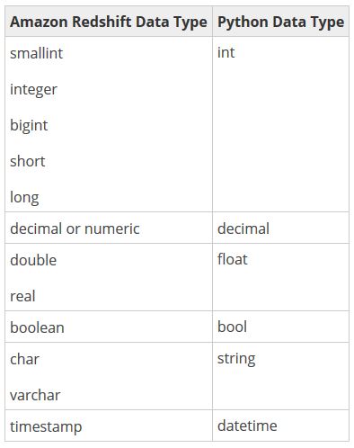
It’s unlikely that any of these mappings will come as much of a surprise, but one additional data type that may come in handy is the ANYELEMENT data type. ANYELEMENT is a polymorphic data type at your disposal that is actually passed to the function when it is called. It’s a data type that lets you take advantage of Python’s inherent duck typing behavior.
Setting up your Amazon Redshift environment
If this is your first Amazon Redshift cluster, follow the instructions from Getting Started with Amazon Redshift to spin up your infrastructure. Many of the existing tools you use for querying databases will probably work in a very similar fashion with Amazon Redshift.
To create a UDF, your account must have USAGE privilege on the Python language. The syntax for Python language usage is:
GRANT USAGE ON LANGUAGE plpythonu TO USER_NAME_HERE;
After a UDF has been created, the owner or a super user can execute it; other users must be granted privileges for each function.
The CMS Open Payments data set contains several files but to follow along with this tutorial, the only file needed is the general payments data. The general payments table you will create contains the payments or other transfers of value not made in connection with a research agreement or research protocol.
To create the table and load it, first download the files from the CMS Open Payments Website and then upload them to your own Amazon S3 bucket. You may find a GUI tool such as S3 Fox Organizer useful for this step as this browser plugin lets you drag and drop the files from CMS into your Amazon S3 bucket.
After you have the data in your own Amazon S3 storage, copy and paste the following SQL script from GitHub: Load the general payment table
For those interested in exploring additional data sets from the CMS Open Payments data, the GitHub repositories below contain similar scripts that create and load tables, but you won’t use them in this post.
- Physician Ownership Information: Information about physicians who have an ownership or investment interest in an applicable manufacturer or applicable group purchasing organization (GPO). Load the identified ownership and investment interest information
- Research Payments: Payments or other transfers of value made in connection with a research agreement or research protocol. Load the identified research payments
- Load the supplementary physician information
Let’s explore!
The general payments data breaks out each physician and type of payment per row. As soon as I saw this data, I wanted to know: Did any physician accept more than a million dollars just in these general payments during the first half of 2013? Note: this first release of data is limited to the first half of 2013.
A simple SQL query churns through the 2.7 million records in just a couple seconds and tells you that there are 20 physicians on that list.
SELECT physician_profile_id,
sum(total_amount_of_payment_usdollars) AS total_general_payments
FROM cms.oppr_all_dtl_gnrl_12192014 gnrl
WHERE physician_profile_id <> ''
GROUP BY physician_profile_id
HAVING sum(total_amount_of_payment_usdollars) > '1000000'
Of course, this may lead to the next question, what type of doctors are these? If you just look at the breakdown of those 20 physicians, it appears that most fall into some type of osteopathic or behavioral health field. You may have some preconceived notations as to why these types of specialties accept more money, but is it a universal truth that these type of physicians tend to accept more in payments or are these simply the million dollar outliers?

To review that question, you can quickly pull an average of all the specialties. However, when you compare the overall average next to the number of actual payments for each specialty, a problem becomes apparent.
SELECT physician_specialty,
avg(total_amount_of_payment_usdollars) AS average_general_payments,
count(*) as number_of_payments
FROM cms.oppr_all_dtl_gnrl_12192014 gnrl
WHERE physician_specialty <> ''
GROUP BY physician_specialty
ORDER BY
AVG(total_amount_of_payment_usdollars) DESC
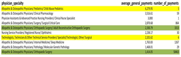
The average payment for a physician in child abuse pediatrics is the highest average, but there are only five samples. Technologists also have a pretty high average, but only six samples (see yellow highlights). Meanwhile, orthopedic surgery has over fifty-eight thousand samples. Is this really a fair comparison?
This is a common problem with financial data, as it often contains large variations such as these. Using a median to eliminate the outliners can help. But often, as data scientists, we want to know more than a simple median, so this is the point in the analysis when SQL functionality starts to become limiting and you pull the data set into a package like SAS, Python, or R in order to run separate statistics. Depending on the setup, you may even need to export your data set, detaching it from your large clustered processing database and potentially limiting your access to future data updates.
However, you can preform your statistical analysis from within your data warehouse using Python UDFs, and, if needed on an ongoing basis, schedule this query just like any other SQL query.
Python UDFs to the rescue
I’m sure many readers of this blog would approach this problem a variety of ways using cool new machine learning algorithms but I’m going to reach back into my high school statistics class and approach this analysis by looking at the Z scores.
As a quick refresher, a Z-test is used to test whether the average of a sample differs significantly from a population mean. In traditional analysis, a T-test is another measure for when a limited sample size is available. In a “big data” world, you have the ability to use a Z-test instead, as you have the data for the entire relevant population. A Z-test is just one of many basic statistical tests that have started to resurface in the cloud because so many of the previous limitations related to storage and computation power are removed.

This simple Z-score calculation can easily be mapped to a Python UDF:
create function
f_z_test_by_pval
(alpha float, x_bar float,
test_val float, sigma float, n float)

--An independent one-sample z-test
--is used to test whether the average
--of a sample differs significantly from a population mean.

--INPUTS:
-- alpha = significant level which we will
--accept or reject hypothesis
-- x_bar = sample mean
-- test_val = specified value to be tested
-- sigma = population standard deviation
-- n = size of the sample

RETURNS varchar
--OUTPUT:
--Returns a simple "Statistically significant"
--or "May have occurred by random chance".
--In a real analysis, you would probably use the
--actual Z-scores but this makes
--for a clean and easy interpretable demo.
STABLE
AS $$

 import scipy.stats as st
 import math as math

 #Z scores are measures of standard deviation.
 #For example, if this calculation returns 1.96,
 #it is interpreted
 #as 1.96 standard deviations away from the mean.
 z = (x_bar - test_val) / (sigma / math.sqrt(n))

 #The p-value is the probability
 #that you have falsely rejected the null hypothesis.
 p = st.norm.cdf(z)

 #in a Z test, the null hypothesis
 #is that this distribution occurred due to chance.
 #When the p-value is very small,
 #it means it is very unlikely (small probability)
 #that the observed spatial pattern is the result
#of random processes, so you can reject the null hypothesis.
Nif p <= alpha:
#rejecting the null hypothesis
   return 'Statistically significant'


 else:
   return 'May have occurred by random chance'


$$LANGUAGE plpythonu;
In addition to preforming statistics in the database, a UDF also gives you the chance to take advantage of the easier string manipulations offered by Python as well.
The physician specialty column is actually a multi-part name that you probably could get better results from if you pulled apart the specific specialties.

The previous list can easily be transformed into a more useable list as follows:

You can transform the list by adding a Python UDF to your database.
create function
f_return_focused_specialty(full_physician_specialty varchar)
--
--INPUTS:
--full_physician_specialty
--Expects the physician separated by "/"

 RETURNS varchar
 --OUTPUT:
 --The focused physician specialty
 -- the rightmost specialty listed.
STABLE
AS $$

    parts = full_physician_specialty.split("/")
    return parts[len(parts) - 1].strip()

$$LANGUAGE plpythonu
Although you could potentially do this with substrings and length functions within SQL, it quickly gets messy and hard to maintain. A Python scalar function makes string processing easy, efficient, and much more readable.
You may have noticed that I prefixed f_ to the name of both of these UDFs. You should do the same with any UDFs that you create. Overloading is allowed so to avoid collisions. Amazon Redshift reserves the f_ prefix exclusively for UDFs. As long as your UDF name starts with f_, you ensure that your UDF name will not conflict with any existing or future Amazon Redshift function.
Running your first function
After you have the UDF created and access is granted, you can call your Python UDF just as you would any other SQL function:
SELECT distinct physician_specialty, f_return_general_specialty(physician_specialty)
FROM cms.oppr_all_dtl_gnrl_12192014
When you run this query, the following steps are performed by Amazon Redshift:
- The function converts the input arguments to Python data types.
- The function executes the Python program, passing the converted input arguments.
- The Python code returns a single value. The data type of the return value must correspond to the RETURNS data type specified by the function definition.
- The function converts the Python return value to the specified Amazon Redshift data type and then returns that value to the query.
Analyzing the data
Armed with Python UDFs, you are now able to find the entire set of statistically relevant physician specialty averages. This single statement calls your SQL and Python processing, saving the full query in a database view to be used later:
Using the view, you can now go back to the question I asked after looking at the million dollar physician list, “Do orthopedic surgeons in general take more money from the drug companies?”
SELECT 'Orthopaedic Surgery', avg_payments, is_valid
 FROM CMS.STAT_RELEVANT_PHYSICIAN_SPECIALTY
 WHERE focused_specality = 'Orthopaedic Surgery'
UNION ALL
 SELECT 'Population', avg(total_amount_of_payment_usdollars) , 'Reference Value'
 FROM CMS.oppr_all_dtl_gnrl_12192014

Well, maybe? An average payment is much higher but the distribution differs enough from the population that it’s possible this value is a created by a chance occurrence such as a handful of surgeons accepting lots of money. Because the Z-score expects a normal distribution, there is a good chance that there are a few outlier payments, causing the average to become skewed.
Conclusion
In this blog post, you learned everything you needed to start implementing scalar Python UDFs in Amazon Redshift. You did this by walking through an analysis of the CMS Open Payments data set, where you found that even though the physicians who accepted the most money from outside influences were mostly orthopedic surgeons, this was not reflective of the entire specialty.
Stay tuned for an upcoming blog post where I will show additional features of Python UDFs, and dive deeper into this data set to find those specialties that do accept more money on average.
In the meantime, you have the ability to leverage the code provided to set up your Amazon Redshift environment and use Python UDFs to ask your own questions of this data.
If you have questions or suggestions, please leave a comment below.
————————————-
Related:
Connecting R with Amazon Redshift