AWS Big Data Blog
Connecting R with Amazon Redshift
Markus Schmidberger is a Senior Big Data Consultant for AWS Professional Services
Amazon Redshift is a fast, petabyte-scale cloud data warehouse for PB of data. AWS customers are moving huge amounts of structured data into Amazon Redshift to offload analytics workloads or to operate their DWH fully in the cloud. Business intelligence and analytic teams can use JDBC or ODBC connections to import, read, and analyze data with their favorite tools, such as Informatica or Tableau.
R is an open source programming language and software environment designed for statistical computing, visualization, and data analysis. Due to its flexible package system and powerful statistical engine, R can provide methods and technologies to manage and process a big amount of data. R is the fastest growing analytics platform in the world, and is established in both academia and business due to its robustness, reliability, and accuracy. For more tips on installing and operating R on AWS, see Running R on AWS.
In this post, I describe some best practices for efficient analyses of data in Amazon Redshift with the statistical software R running on your computer or Amazon EC2.
Preparation
Start an Amazon Redshift cluster (Step 2: Launch a Sample Amazon Redshift Cluster) with two dc1.large nodes and mark the Publicly Accessible field as Yes to add a public IP to your cluster.
If you run an Amazon Redshift production cluster, you might not choose this option. Discussing the available security mechanisms could be a separate blog post all by itself, and would add too much to this one. In the meantime, see the Amazon Redshift documentation for more details about security, VPC, and data encryption (Amazon Redshift Security Overview).
For working with the cluster, you need the following connection information:
- Endpoint <ENDPOINT>
- Database name <DBNAME>
- Port <PORT>
- (Master) username <USER> and password <PW>
- JDBC URL <JDBCURL>
You can access the fields by logging into the AWS console, choosing Amazon Redshift, and then selecting your cluster.
Sample data set
To demonstrate the power and usability of R for analyzing data in Amazon Redshift, this post uses the “Airline on-time performance” (http://stat-computing.org/dataexpo/2009/) data set as an example. This data set consists of flight arrival and departure details for all commercial flights within the USA, from October 1987 to April 2008. There are nearly 120 million records in total, which take up 1.6 gigabytes of space compressed and 12 gigabytes when uncompressed.
Copy the data to an Amazon S3 bucket, in same region as your Amazon Redshift cluster, and create the tables and load the data with the following SQL commands. For this demo purpose, our cluster has a IAM_Role attached to it which has access to the S3 bucket. For more information on allowing Redshift cluster to access other AWS services please go through this documentation.
CREATE TABLE flights(
year integer   encode lzo,
month integer   encode lzo,
dayofmonth integer   encode delta DISTKEY,
dayofweek integer   encode delta,
deptime integer   encode delta32k,
crsdeptime integer   encode lzo,
arrtime integer   encode delta32k,
crsarrtime integer   encode lzo,
uniquecarrier varchar(10)   encode lzo,
flightnum integer   encode lzo,
tailnum varchar(10)   encode lzo,
actualelapsedtime integer   encode bytedict,
crselapsedtime integer   encode bytedict,
airtime varchar(5)   encode bytedict,
arrdelay integer   encode bytedict,
depdelay integer   encode bytedict,
origin varchar(5)   encode RAW,
dest varchar(5)   encode lzo,
distance integer   encode lzo,
taxiin varchar(5)   encode bytedict,
taxiout varchar(5)   encode bytedict,
cancelled integer   encode lzo,
cancellationcode varchar(5)   encode lzo,
diverted integer   encode lzo,
carrierdelay varchar(5)   encode lzo,
weatherdelay varchar(5)   encode lzo,
nasdelay varchar(5)   encode lzo,
securitydelay varchar(5)   encode lzo,
lateaircraftdelay varchar(5)   encode lzo
)
SORTKEY(origin,uniquecarrier);

COPY flights FROM 's3://data-airline-performance/'
IAM_Role '<RedshiftClusterRoleArn>'
CSV DELIMITER ','
NULL 'NA'
ACCEPTINVCHARS
IGNOREHEADER 1;
/*If you are using default IAM role with your cluster, you can replace the ARN with default as below

COPY flights FROM 's3://data-airline-performance/'
IAM_Role default
CSV DELIMITER ','
NULL 'NA'
ACCEPTINVCHARS
IGNOREHEADER 1;
*/
SELECT count(*) FROM flights; /* 123.534.969 */
For these steps, I recommend connecting to the Amazon Redshift cluster with SQLWorkbench/J (Connect to Your Cluster by Using SQL Workbench/J). Be aware that the COPY command executes a parallel load for each file of the data located in Amazon S3, which accelerates the loading process.
Your R environment
Before running R commands, you have to decide where to run your R session. Depending on your Amazon Redshift configuration, there are several options:
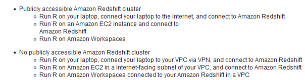
Your IT department or database administrator can provide you with more details about your Amazon Redshift installation.
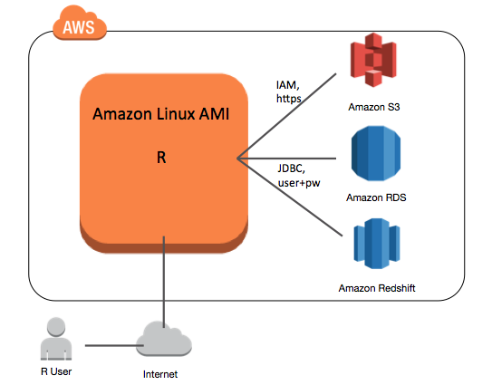
I recommend running R on an Amazon EC2 instance using the Amazon Linux AMI as described in Running R on AWS. The EC2 instance will be located next to your Amazon Redshift cluster, with reduced latency for your JDBC connection.
Connecting R to Amazon Redshift with RJDBC
As soon as you have an R session and the data loaded to Amazon Redshift, you can connect them. The recommended connection method is using a client application or tool that executes SQL statements through the PostgreSQL ODBC or JDBC drivers.
In R, you can install the RJDBC package to load the JDBC driver and send SQL queries to Amazon Redshift. This requires a matching JDBC driver. Choose the latest JDBC driver provided by AWS (Configure a JDBC Connection).
This driver is based on the PostgreSQL JDBC driver but optimized for performance and memory management.
install.packages("RJDBC")
library(RJDBC)

# download Amazon Redshift JDBC driver
download.file('http://s3.amazonaws.com/redshift-downloads/drivers/RedshiftJDBC41-1.1.9.1009.jar','RedshiftJDBC41-1.1.9.1009.jar')

# connect to Amazon Redshift
driver <- JDBC("com.amazon.redshift.jdbc41.Driver", "RedshiftJDBC41-1.1.9.1009.jar", identifier.quote="`")
# url <- "<JDBCURL>:<PORT>/<DBNAME>?user=<USER>&password=<PW>
url <- "jdbc:redshift://demo.ckffhmu2rolb.eu-west-1.redshift.amazonaws.com
:5439/demo?user=XXX&password=XXX"
conn <- dbConnect(driver, url)
The URL is a combination of the JDBC URL provided by the AWS console, and the user and password passed as arguments. As soon as you have a connection to the cluster, you can submit SQL commands to get information about the database and different SQL queries to access data.
# list tables
dbGetTables(conn)
dbGetQuery(conn, "SELECT table_name FROM information_schema.tables WHERE table_schema = 'public'")

# get some data from the Redshift table
dbGetQuery(conn, "select count(*) from flights")

# this is not a good idea – the table has more than 100 Mio. rows”
# fligths <- dbReadTable(conn, "flights")

# close connection
dbDisconnect(conn)
The RJDBC package provides you with the most flexibility and the best performance. You should use this package for all your SQL queries to Amazon Redshift. Unfortunately, you have to implement everything by using SQL commands. Packages such as RPostgeSQL or https://github.com/pingles/redshift-r do not use the optimized Amazon Redshift JDBC driver but will also work. In some special cases, such as running SQL queries on big tables, you will see some performance reduction. The RedshiftRDBA code on Github is not for querying data in Amazon Redshift; this repository provides useful R functions to help database administrators analyze and visualize data in Amazon Redshift system tables.
Efficient analysis using the dplyr package
The dplyr package is a fast and consistent R package for working with data frames like objects, both in memory or on databases. This avoids having to copy all data into your R session, and allows you to load as much of your workload as possible directly on Amazon Redshift. This package provides connections to many database systems. You have to create a connection to Amazon Redshift via the RPostgreSQL package.
First, connect to your Amazon Redshift cluster.
# now run analyses with the dplyr package on Amazon Redshift
install.packages("dplyr")
library(dplyr)
library(RPostgreSQL)
#myRedshift <- src_postgres("<DBNAME>",
#	host = "<ENDPOINT>,
#	port = <PORT>,
#	user = "<USER<",
#	password = "<PW>")
myRedshift <- src_postgres('demo',
host = 'redshiftdemo.ckffhmu2rolb.eu-west-1.redshift.amazonaws.com',
port = 5439,
user = "markus",
password = "XXX")
Then, create a table reference using the function tbl(). This means you are creating an R object which points to the table in the Amazon Redshift cluster, but data is not loaded to R memory. As soon as you execute R functions to this R object, SQL queries are executed in the background. Only the results are copied to your R session.
# create table reference
flights <- tbl(myRedshift, "flights")

# simple and default R commands analyzing data frames
dim(flights)
colnames(flights)
head(flights)

#the summarize command reduces grouped data to a single row.
summarize(flights, avgdelay=mean(arrdelay))
summarize(flights, avgdelay=max(arrdelay))
Without loading data to R directly, you can execute great analyses on Amazon Redshift using R. The downside of the functional nature of dplyr is that when you combine multiple data manipulation operations, you have to read from the inside out. In many cases, the R function arguments may be very distant to the function call. The %>% operator provides an alternative way of calling dplyr functions that you can read from left to right, and is very intuitive to use.
Now do some advanced analysis. If you are interested in all flights that make up more than 60 minutes during their flight, use the following example:
flights %>%
filter(depdelay-arrdelay>60) %>%
select(tailnum, depdelay, arrdelay, dest)
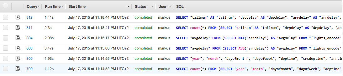
You can get this result in seconds and, if you check your Amazon Redshift queries list, you see that several SQL commands were executed.
You may also be interested in the delay of flights grouped by month and destination. Be aware that if you store your dplyr operations into a new object, “res”, the query to Amazon Redshift is not executed. When you use the “res” object, then the query is executed. This reduces runtime and workload for your Amazon Redshift cluster.
res <- flights %>%
group_by(month, origin) %>%
summarize(delay=mean(arrdelay))

dres <- as.data.frame(res)
ggplot(aes(month, delay, fill=origin), data=dres) + geom_bar(stat="identity", position="dodge")

I found some nice results in the “Airline on-time performance” data set. The bar plot visualizes the average delay per month over all years (21 years of flight data), and only shows the values for three big airports: JFK, ORD, and PHL. The arrival delay over month is very similar for the big airports in the US, which means that there are very low local influences. Furthermore, I expected to see higher delays in winter instead of the actual highest delay times in June, July, and August.
Amazon Redshift database administrator tips
It might be a good idea to define a separate query queue for your data scientists connecting to Amazon Redshift via R (Defining Query Queues). A separate queue can avoid long-running R SQL queries that influence the execution time of your production queries.
Furthermore, the Amazon Redshift Utils (https://github.com/awslabs/amazon-redshift-utils) published at github provide a collection of scripts and utilities that will assist administrators in getting the best performance possible from Amazon Redshift. The “perf_alter.sql” script might be useful to monitor performance alerts related to R queries.
For all my demo code in this post, I used the Amazon Redshift superuser created during the Amazon Redshift launch process. For security and data protection, I recommend that you create separate Amazon Redshift users (Managing Database Security) for all R developers, and grant permissions based on the required operations and tables.
Summary
The statistical software R enables you to run advanced analyses on your data located in the managed, highly available, and scalable Amazon Redshift data warehouse. The RJDBC package provides fast and efficient access via SQL commands and the dplyr package allows you to run efficient analyses without any SQL knowledge.
If you have questions or suggestions, please leave a comment below.
————————————
Related:
